How Yo Make Each Level.of Graph.different Color
Visualization with Plotly.Express: Comprehensive guide
One dataset and over 70 charts. Interactivity and animation often in a single line of code
![]()

I frequently come up with an ideal visualization and then struggle to code it. It would be to the point, expressive, and easy to interpret, but it's impossible to create. When I found Plotly it made plotting, well, much easier.
Plotly.Express, first introduced in version 4.0.0 is a high-level abstraction to Plotly API optimized to work perfectly with data frames. It's very good, though not flawless. I see the biggest gap in the number of examples or links to the API documentation. That's why I have decided to use my experience with the library to write a guide.
To run the chart and exercises, please use the Plotly Express — Comprehensive Guide.ipynb notebook on Github. All the code in this article is in python.
Table of contents:
- Installation — and dependencies
- Plotly.Express syntax — one line of code
- Data matters — should we pre-processed data into a wide or a long-form?
- Line Chart — used for a gentle introduction, understanding the input data and parameters we can pick to customize the chart
- Layout — templates and styling
- Annotation — to help you describe the data
- Chart types — scatter, bar, histogram, pie, donut, sunburst, treemap, maps with choropleth,
- Interactions — Buttons changing the chart
- Pitfalls — and other things to improve
- Summary of the documentation
Installing Plotly Express
Plotly.Express is a regular part of the Plotly python package, so the easiest is to install it all.
            # pip
pip install plotly            # anaconda
conda install -c anaconda plotly
Plotly Express also requires pandas to be installed, otherwise, you will get this error when you try to import it.
            [In]: import plotly.express as px
[Out]:              ImportError: Plotly express requires pandas to be installed.
There are additional requirements if you want to use the plotly in Jupyter notebooks. For Jupyter Lab you need jupyterlab-plotly. In a regular notebook, I had to install nbformat (conda install -c anaconda nbformat)
Plotly Express syntax — One line of code
Plotly.Express offers shorthand syntax to create many chart types. Each comes with different parameters and understanding the parameters is the key to Plotly.Express charm. You can create most of the charts with one command (many advertisers say one line, but due to PEP8 recommending up to 79 characters per line, it's usually longer).

            import plotly.express as px            # syntax of all the plotly charts
px.chart_type(df, parameters)
To create a chart with Plotly.Express you only type px.chart_type (many types will be introduced later). This function consumes a dataframe with your data df and the parameters of the chart. Some parameters are chart specific, but mostly you input x and y values (or names and values e.g. in the case of pie chart). You label the datapoints with text and split into categories (separate lines, bars, pie's sectors) by color, dash or group. Other parameters let you influence the colors, split to subplots (facets), customize the tooltips, scale and range of the axes and add animations.
Mostly you assign the plot into a variable so that you can influence the setup of the graph elements and the layout.
            fig = px.chart_type(df, parameters)
fig.update_layout(layout_parameters or add annotations)
fig.update_traces(further graph parameters)
fig.update_xaxis() # or update_yaxis
fig.show()
The Dataset
Even though plotly comes with some integrated datasets, they were used in many existing examples, so I've picked my favorite dataset about the number of tourists visiting each country and the money they spent on their vacation. The dataset is available by World Bank under CC-BY 4.0 license.
As with every dataset, even this one needs some pre-processing. What is very annoying about the tourism dataset is that it mixes values per country with regional aggregates. The pre-processing is simple (see code) and it's important to say that the dataset comes in a wide form.
The Data Matters (wide and long data frame)
All data frames can be transformed into many forms. A data table can be wide with information stored in many columns or long with data in rows. Luckily python and pandas library allows converting between these with ease using DataFrame.T to turn rows into columns, melt() for melting columns into long data frame and pivot() and pivot_table() to do the opposite. Nicolas Kruchten explains it well that in his Beyond "tidy" article, so I'll not spend more time discussing it here. You can also see all the data operations in the commented notebook on the Github.
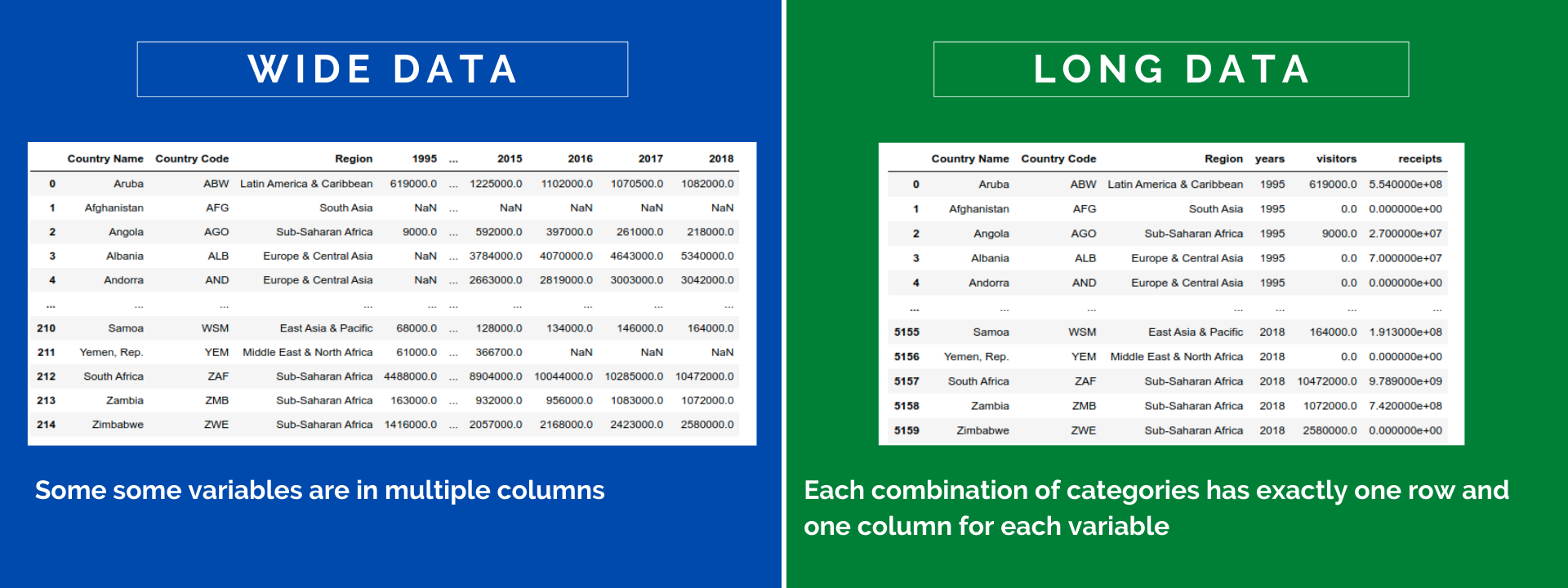
Plotly.Express works the best with the long data. It's designed to accept one column as a parameter. Categorical columns influence the elements (lines, bars …) and can be differentiated by styles while value columns affect the size of the elements and can be displayed as labels and in tooltips.
Limited possibilities of the wide data
You can use Plotly express with wide data as well, but the use-cases are limited. Let's explore what you can do with the wide dataset and its limits.
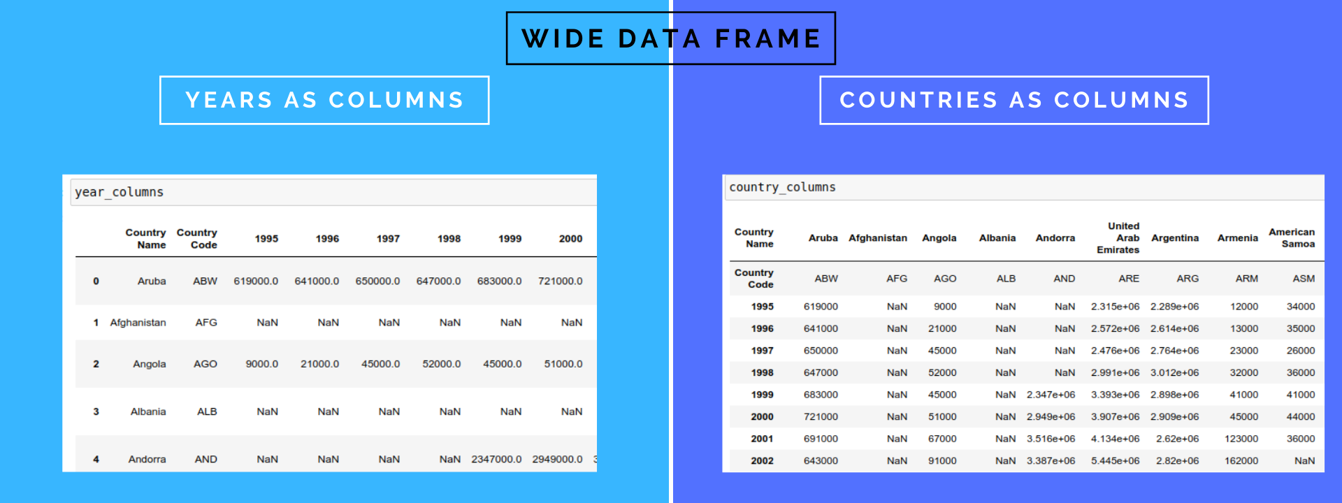
The first parameters are almost the same for all the charts — the dataset, x and y. X and y can be the names of the columns in the dataframe, padnas.Series or an array. Our tourism dataset comes in the wide form with many columns. Since we have years as columns and Country Names as rows, we switch between them using pandas.DataFrame.T because Plotly.Express API works with columns.
Below, the three ways to draw a chart are equivalent. Check yourself, but I think the first one makes the most sense. If you use a column or a series, its name appears as an axis label, while in the case of an array you must add the label manually.
"""our dataset comes as a wide dataset with years as column. To turn the country names into the columns, we must set them as index and transpose the frame."""
country_columns = year_columns.set_index("Country Name").T # 1. I had to reshape the data by transposing
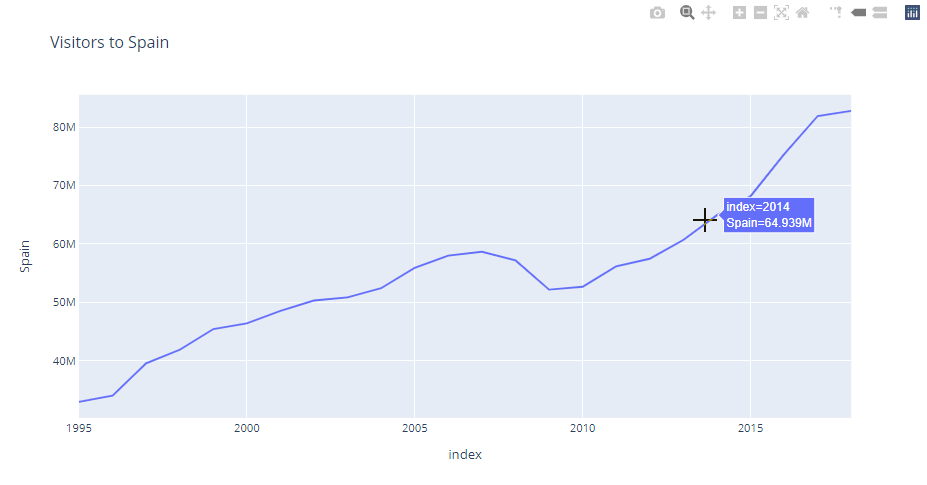
px.line(country_columns
,y="Spain"
,title="Visitors to Spain") # 2. you can specify the value as pandas.Series as well
px.line(country_columns,
y=country_columns["Spain"],
title="Visitors to Spain") # 3. or any array. In this case you must specify y-label.
px.line(country_columns,
y=country_columns["Spain"].to_list(),
labels={"y":"Spain"},
title="Visitors to Spain")
Having a dataset which contains several descriptive columns
Country Name,Country Code,Region, mixed with data columns like visits in1995,1996—2018shows one of the benefits of Plotly. It's clever enough to consider only the columns with values and silently ignores the rest.
You can easily pick multiple columns to your chart.
px.line(country_columns, y=["Spain","Italy","France"]) 
Limits of the wide data frame
In Plotly, you can do some operations with a dataset containing many columns, but the real power of the library lies in the long data. The reason, most of the parameters accept exactly one column. It can have several distinct (usually categorical) values and plotly do its magic on them, but there cannot be more than one column. The following code leads to an error:
            [In]:
try:
              px.line(country_columns, y=["Spain","Italy","France"],
              # trying to label the line with text parameter
              text=["Spain","Italy","France"])            except Exception as e:
              print(e)            [Out]:              All arguments should have the same length. The length of argument `wide_cross` is 25, whereas the length of  previously-processed arguments ['text'] is 3
You can try to pick one of the columns, but the result is a complete fail. Line charts for Italy and France annotated with the values about visitors to Spain. A catastrophe.
            px.line(country_columns, y=["Spain","Italy","France"],
text="Spain") 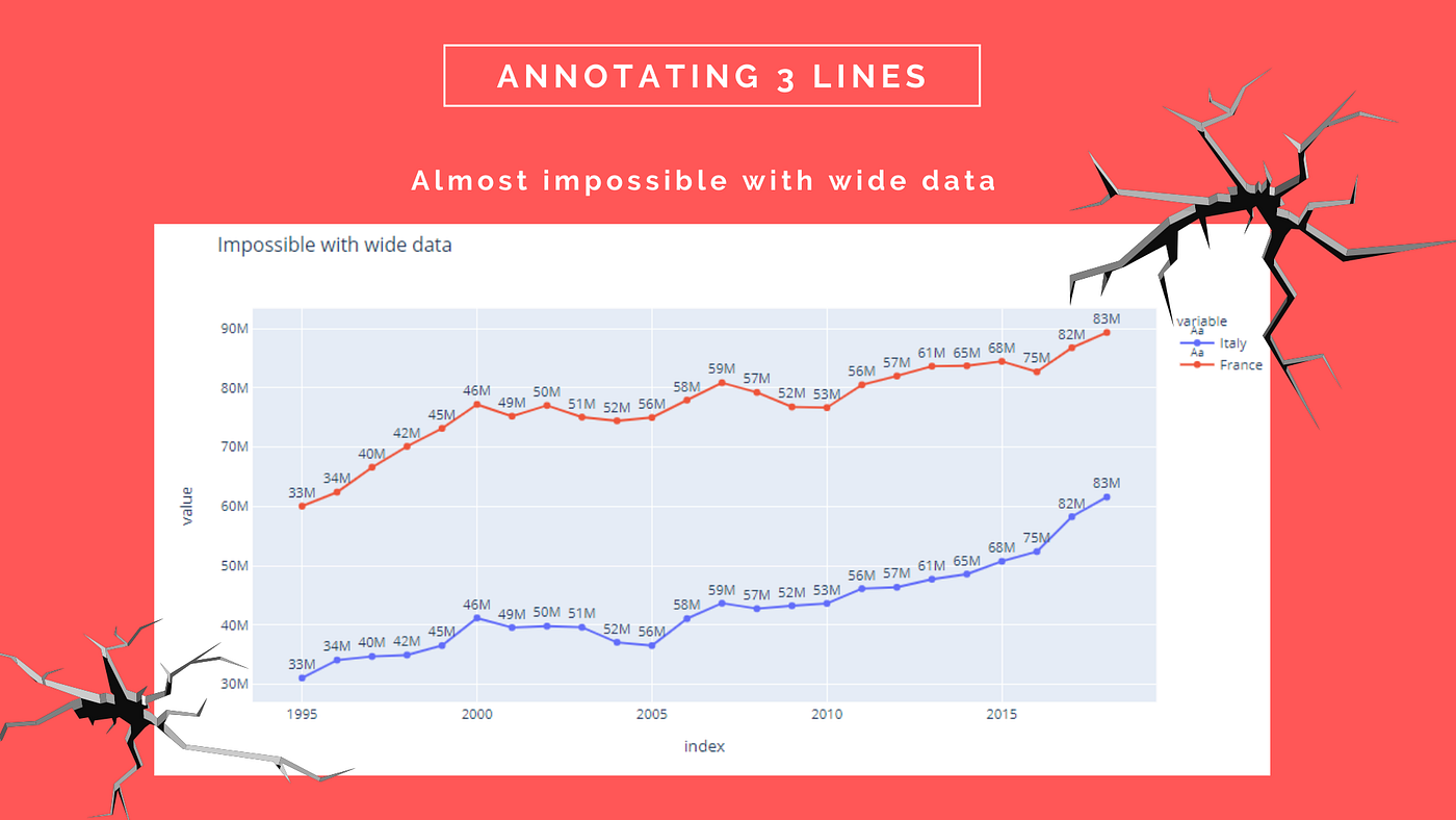
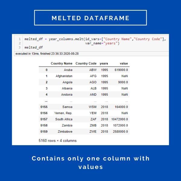
The Long data — Metled DataFrame
There's nothing wrong with Plotly. To exploit the parameters you must use a long data frame. From a wide dataset, you get it using .melt() function. I'll also filter only 3 countries not to have the chart too crowded.
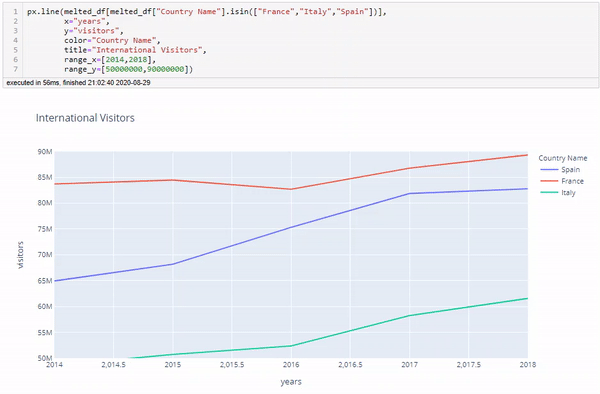
            spfrit = melted_df[melted_df["Country Name"].isin(["Spain","Italy","France"])]            px.line(spfrit,
              x="years",
              y="visitors",
              color="Country Name",
              text="visitors",
              title="International Visitors")
Assigning a single column to each parameter let plotly determine the rest:
-
x— x axis contains all distinct values from theyearcolumn (1995 to 2018) -
y— y axis cover the whole range fromvisitorscolumn -
color— set three different colors to distinct values in theCountry Namecolumn (France, Italy and Spain) -
text— label each line with a value of the visitors in each year
Line Chart
Let's explore the basic line chart to admire how easily you can create visualizations with Plotly. Each Plotly's chart is documented in several places:
- The chart type page — e.g. Line Charts in Python — showing the most common examples
- Python API reference — e.g. express.line — describing all the parameters you can use
In the previous section, you have seen that a line chart needs x and y values which can come in three forms, but the most common for Express is to use the column name to specify which data frame's column control the graph's functionality.
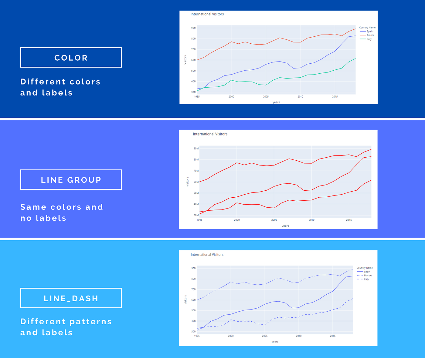
Line chart parameters colors, dashes, groups
color — is the key parameter for many chart types. It splits the data into groups and assigns them distinct colors. Each of the groups forms an element, in the case of a line chart, it's a separate line. The colors are assigned to each line unless you set the exact colors using the following parameters.
color_discrete_sequence — to choose pre-defined colors of the lines, e.g. color_discrete_sequence = ["red","yellow"]. If you provide fewer colors than the number of your series, Plotly will assign the rest automatically.
color_discrete_map — allowing the same as above but in the form of a dictionary assigning color to a specific series. color_discrete_map = {"Spain":"Black"}.
line_dash — similar to color it only changes the dash pattern instead of color
line_group — similar to color, it's used to distinguish the value (category) which separates the lines, but in this case, all will have the same color and no legend will be created for them.
Tooltips
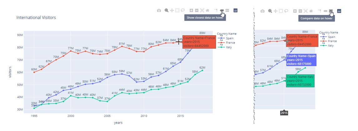
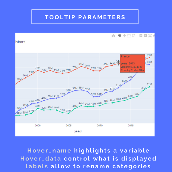
Plotly inherently brings interactive tooltips. Above you can see that you can switch between closest and all data tooltips. There are also parameters to customize these textboxes even more — hover_name highlights the value of this column on the top of the tooltip. hover_data allow to True/False the categories or values which should appear on the tooltip. labels param let you rename these categories.
Other useful parameters
We have created 3 lines with different colors per country. Changing thecolor parameter to facet_col or facet_row to creates 3 separate charts. Keeping both the facet and the color ensures that each line has a distinct color. Otherwise, it would be the same. You can zoom into one of the plots and others will zoom too.
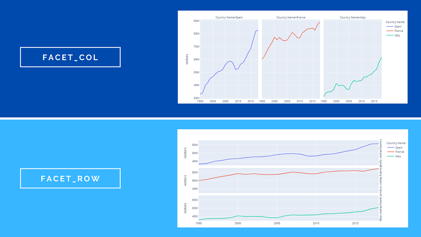
Faceted subplots are also the only way how to create subplots with Plotly.Express. Unfortunately, you cannot just create a line chart on the top of a bar chart with Express. You need Plotly's lower-level API.
range_x and range_y parameters allow to zoom into the chart. You can always use the interactive controllers to see the full range of data.
log_x and log_y set to True will change these axes to be log-scaled in cartesian coordinates.
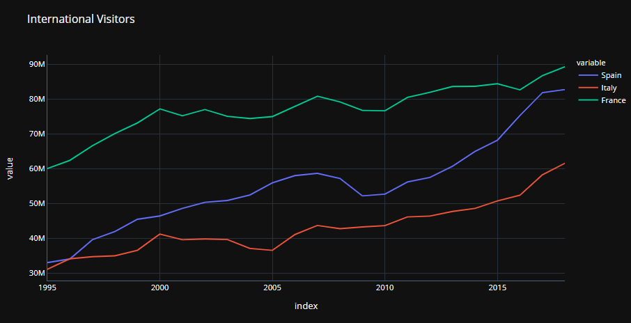
Animations
And finally, we're getting to the parameters which made plotly.Express popular. The animations. The parameter animation_frame points to a column that is used to differentiate the animation frames. I had to update the dataset a bit to create this animation. Column years_upto contains all the historical data. See the notebook on the github for more info.
            year_upto   year country visitors
1995        1995 ESP     30M
1996        1995 ESP     30M
1996        1996 ESP     33M
1997        1995 ESP     30M
1997        1996 ESP     33M
1997        1997 ESP     37M            # then I use `year_upto` as the animation_frame parameter
px.line(spfrit,
              x="years",
              y="visitors",
              color="Country Name",
              title="International Visitors",
              range_x=[1995, 2018],
              range_y=[25000000,90000000],
              animation_frame="year_upto")

The Layout and styling
Before we move to introducing a whole range of Plotly chart types, let's explore basic techniques on how to update the axes, legend, titles, and labels. Plotly prepared a styling guide, but many chart types allow just some styling options which are hard to figure out from the documentation.
Every plotly chart is a dictionary
On background, each graph is a dictionary. You can store the chart into a variable, commonly fig and display this dictionary using fig.to_dict().
            [In]: fig.to_dict()
[Out]:
{'data': [{'hovertemplate': 'index=%{x}<br>Spain=%{y}<extra></extra>',
              'legendgroup': '',
              'line': {'color': '#636efa', 'dash': 'solid'},
              'mode': 'lines',
...
Thanks to that you can update the chart using 3 ways.
- using
fig.udpate_layout() - using a specific parameter eg.
fig.update_xaxis() - by changing the background dictionary
Each of them gets tricky sometimes because you have to really dig into the documentation to understand some of the parameters. Each of the parameters can be updated using 4 different ways.
            # Four options how to update the x-axis title
# 1.and 2. using update_layout
fig.update_layout(xaxis_title="X-axis title",
              xaxis = {"title": "X-axis title"})            # 3. using update_xaxes
fig.update_xaxes(title_text="X-axis title")            # 4. by modifying the dictionary
fig["layout"]["xaxis"]["title"]["text"] = "X-axis title"            # in the end you show the plot
fig.show()
Templates
The easiest way to style the chart is by using pre-defined templates. Plotly comes with several build-in templates including plotly_white, plotly_dark, ggplot2, seaborn or your can create your own template.
Yaxis and Xaxis
We can update the other parameters one by one. Looking just on axes for 2D charts with 2-dimensional Cartesian axes, you have many options for what to change (see plotly python). Let's look at the most important.
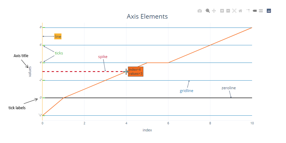
-
visibility— is the axis visible -
color— of all elements line, font, tick, and grid -
title— axis title (parameters: text, font, color, size, standoff) -
type— axis types: linear, log, date, category or multicategory -
range— value range of the axis (autorange, rangemode, range) -
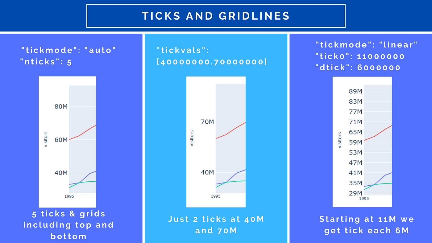
ticks— ticks and corresponding gridlines (tickmode, tickvals, nticks, tickangle, etc.) -
spike— line drawn between the point and axis
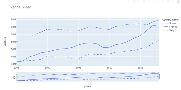
One cool option for the x-axis is the range slider. You set it up using fig.update_xaxes(rangeslider_visible=True) and it highlights the part of the plot you zoom in. It's very useful with the time series.
Later I'll broach some pitfalls with the ticks and the difference between a category and linear mode, but now, let's move on and have a look at another important feature used to highlight key ares of the chart.
Annotations
Adding specific text into the chart is called annotating. There are several basic use cases of annotation:
- To highlight point(s)
- To describe/highlight an area
- To label a desired point
- Instead of a legend
We will show all 4 practices in the following image. We label the start point value outside of the chart, annotate a breakpoint, place a message about tourism growth and legend the lines on their right end.
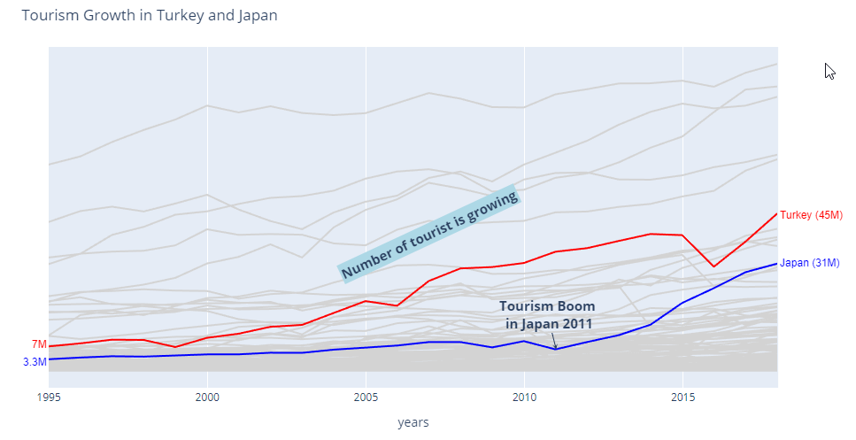
The chart above was tricky. Plotly orders the lines in the order of appearance, so the data had to be sorted. Also Express struggle a bit with assigning color from the long dataframes (I know I was saying that long dfs are the ideal solution, they are not 100%), so I had to do little magic you can study in this gist or read the detailed guideline in Highlighted line chart article.
You might also notice, that with increased number of lines, Plotly automatically switched to WebGL format proven to improve the usability of the JavaScript plots with many data points.
[In]: type(fig.data[0])
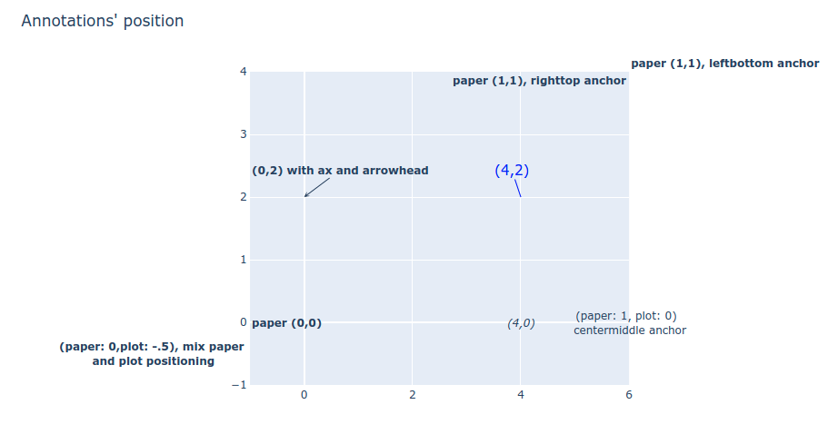
[Out]: plotly.graph_objs._scattergl.Scattergl Regarding the annotations, you have several options on how to influence their positions. You set all the annotations as a list in .fig.update_layout(..., annotations=[]) It contains a list of dictionaries specifying the parameters of the labels:
            annotations = \
[{"xref":"paper", "yref":"paper", "x":0, "y":0.15,
              "xanchor":'right', "yanchor":"top",
              "text":'7M',
              "font":dict(family='Arial', size=12, color="red"),
              "showarrow":False}, ... other annotations ...]
You can specify the position, font, and an arrow between the label and the data point. The coordinates x and y of the text can either refer to the plot or the paper-canvas. "xref"="paper" (0,0) is the bottom left corner of the plot area and (1,1) is the top right corner. Within the chart, you reference using the x and y values on the axis (e.g. year 2008 and 10_000_000 visitors).
The position also depends on the anchor (top-middle-bottom, left-center-right), offsets and adjustments. Each annotation can be modified by setting its font or HTML tags can be applied on the text like <b> or <i>.
Bar Chart
Now when we know how to create a chart, update its layout, and include annotation, let's explore another typical chart types. We will start with the bar chart which is another popular method of how to display trends and compare numbers in categories. The syntax remains the same one-liner:
px.bar(df, parameters) The bar chart API documentation describes all the parameters. Most of the parameters are the same as for the line chart.
Barmode
There are three types of modes bar chart comes in. Relative which stacks the bars on the top of each other. overlay drawing bars on the top of one another with lower opacity and group for clustered columns.

Colors
Like lines, the bars can be colored to make an impactful visualization. You can use color parameter set to a category (e.g. Country Name) to color each bar with a different color from a palette or setting color to a value (e.g. visitors) to differentiate the color by the scale of a tourist visit.
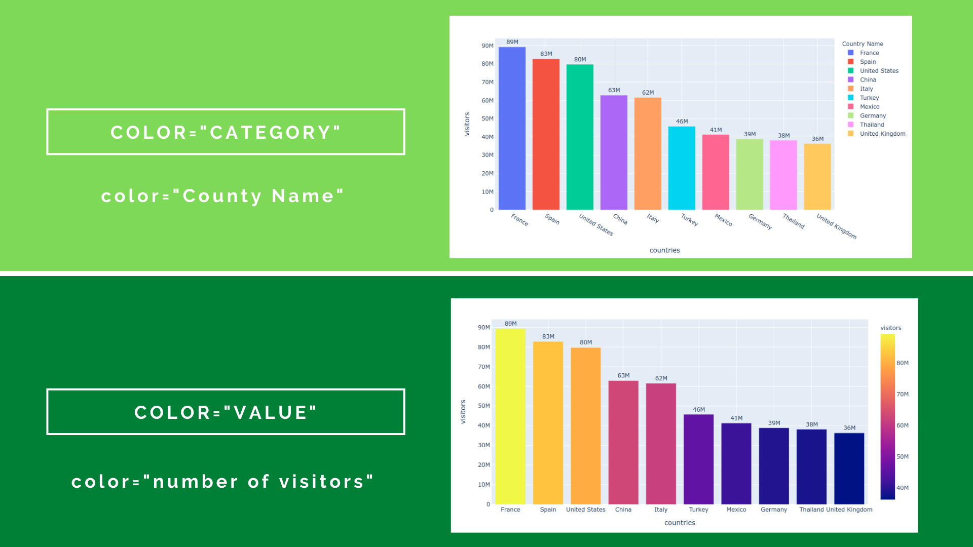
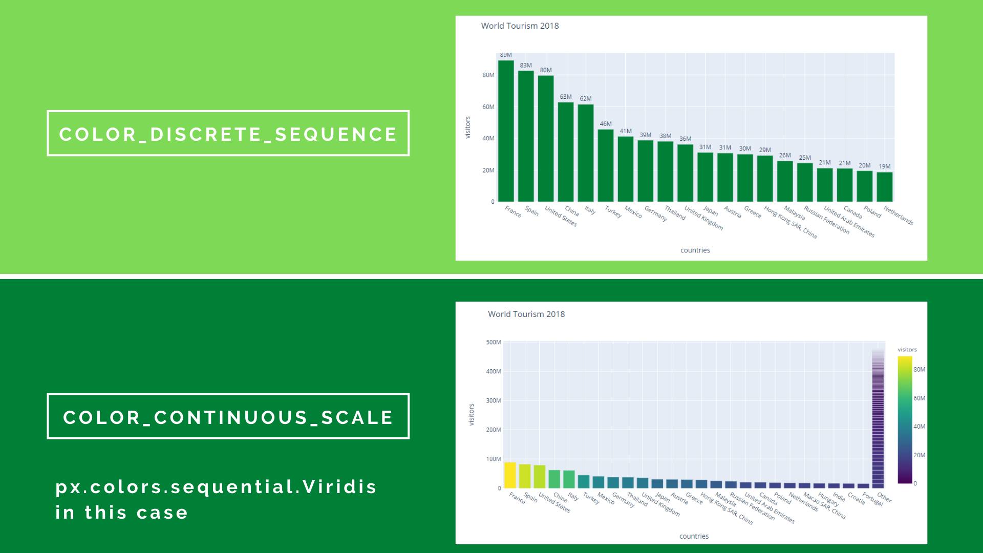
All the bars can have the same color with color_discrete_sequence and you can apply different color based on the the scale — number of visitors in our case using color_continuous_scale.
Combining line a bar chart
One thing Plotly.Express is really bad in are charts with combined types. You can somehow add bars to the line chart, but you cannot do the opposite. And the result, yeah, make your own opinion.
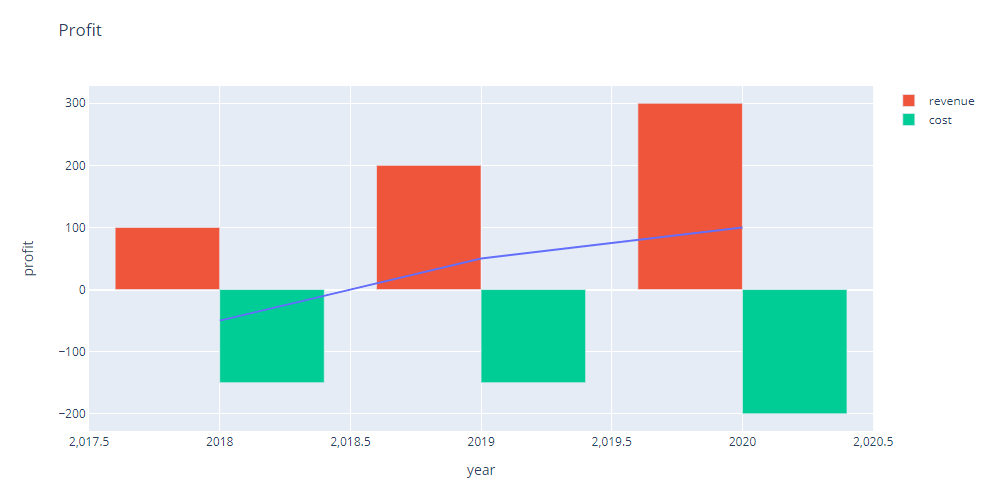
If you want to shine with some mixed typed graph, use lower level API of Plotly. That can do much more than Express, but the code is longer.
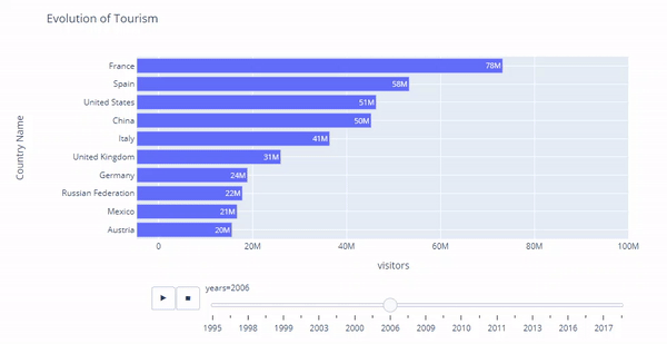
Animated Bar Chart
Parameter animation_frame let you do the animation magic. But it's not all gold that glitters. You have to set up the same range for all frames [0–100M], but the chart is still jumping, because despite y-axisstandoff to make there enough space, longer country names still move the chart. Also, the labels which were originally outside of the bars got inside them on the second animation frame. It would require a bit more customization to be perfect.
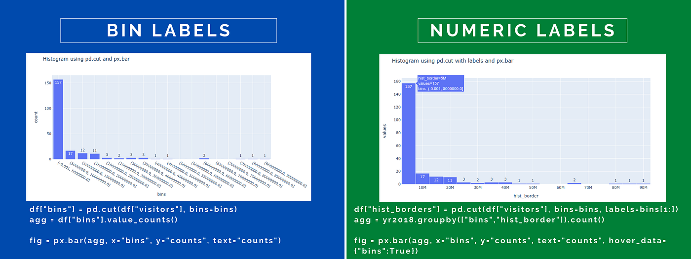
Histogram
A histogram is technically a bar chart without gaps between the bars. The power of the histogram is that it automatically splits the data into bins and aggregate the values in each bin. But it doesn't do it very well (yet).
Histograms use similar parameters like bar charts. You can split the bins by categories using color.
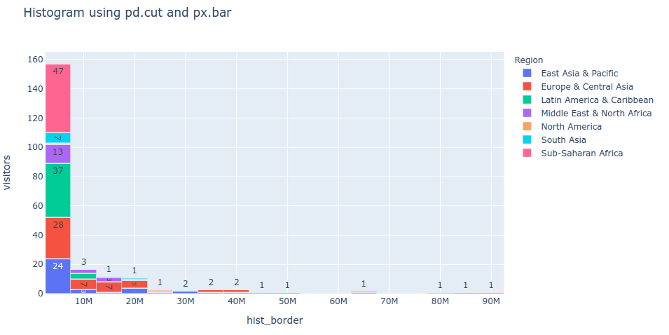
Histograms also have their own parameters. nbins influence the number of bins.

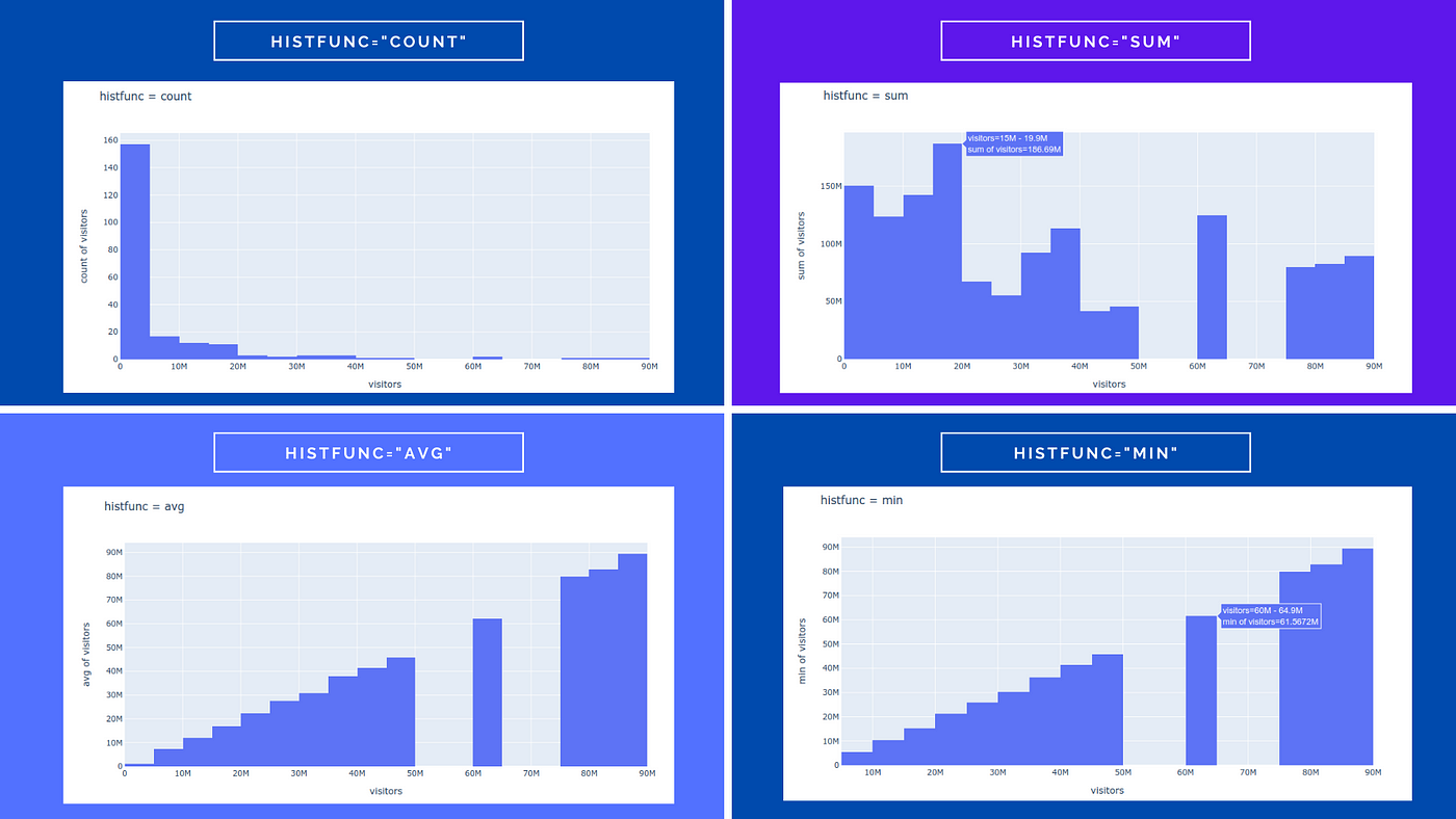
Histfunc allow changing the aggregation function. Of course, when you do average, min or max on the bin between 10 and 20, the values will lie inside this range, so such a histogram will create a stair pattern.
You can also create a cumulative histogram by setting cumulative=True.

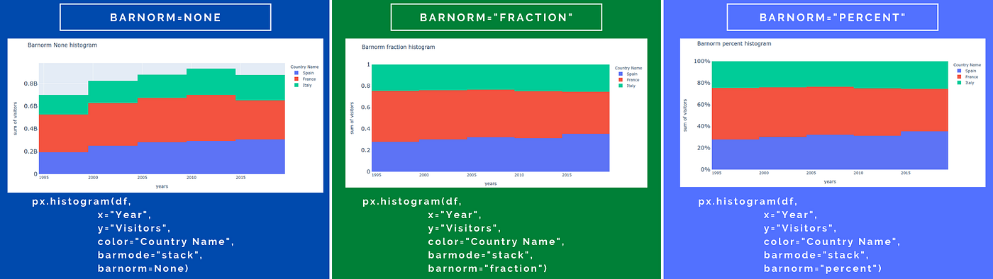
Barnorm let you normalize the values in each bin to be between 0–100%. Barnorm parameter normalizes in each bin, so the values 10, 40, 50 forms 10%, 40% and 50% while 100, 400 and 500 create the chart of the same height also being 10%, 40% and 50%. You have the option to display percent with barnorm="percentage" or decimal numbers with barnorm="fraction".
Histnorm parameter is very similar, but the normalization is not inside one bin, but for each category across all the bins. If your category A appears twice within the first bin, 5 times in the second bin and 3 times in the last one, the histnorm will be 20%, 50% and 30%.
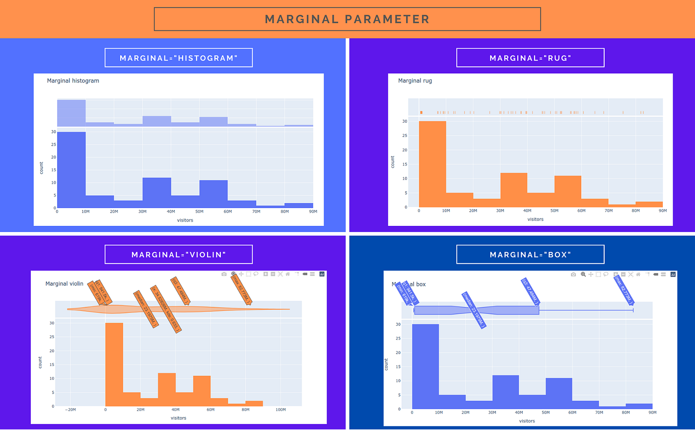
The specific parameter to the histogram (and the scatter plots) is a marginal chart. It let you create a small side chart showing details of the distribution of the underlying variable. There are four types of marginal charts — rug, histogram, box and violin creating the side plots with the same name.
Quite often you need more control over the binning and you rather calculate the bins yourself and plot them using px.bar with fig.update_layout(bargap=0).
Pie Chart
Another option how to achieve a great visualization is to use the pie chart.
            # syntax is simple
px.pie(df, parameters)
When you read the docs you will learn that pie chart doesn't have x and y axes but names and values.
Pull pie's traces
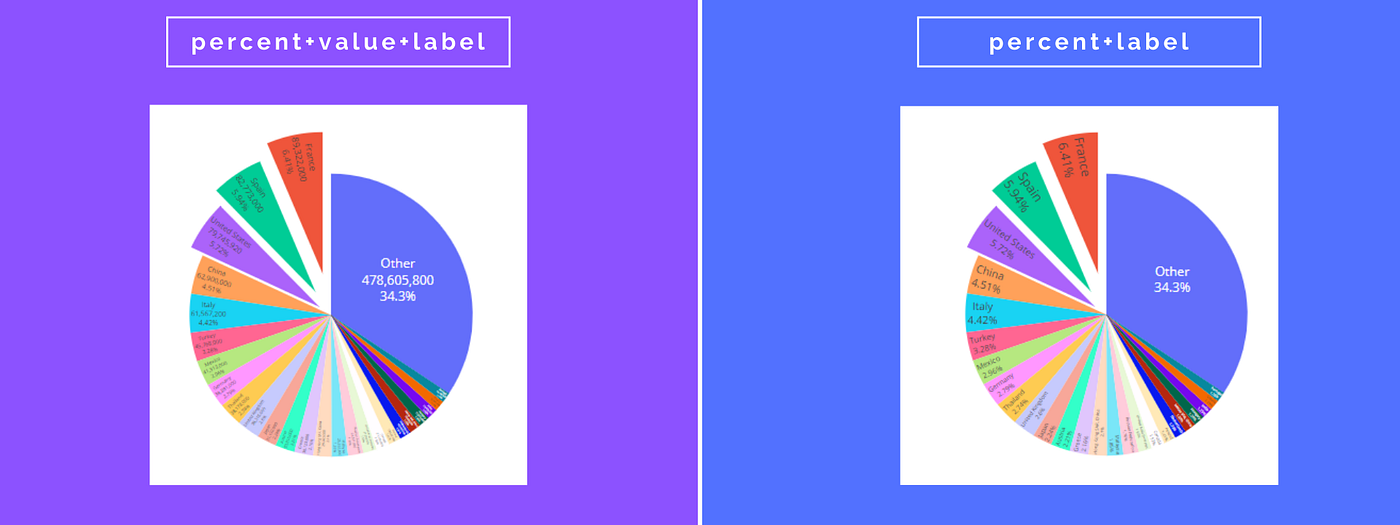
One of the cool things is that you can pull some slices of the plot to highlight them. It's not a parameter of the .pie() but you can add it using fig.update_traces(). Text configuration of the traces also allows to set up the labels as percent, value or label (or any combination of the three e.g. fig.update_traces(textinfo="percent+label"))
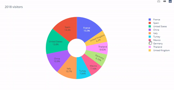
Donut chart — Hole parameter
Pie chart is a bit playful and using hole param you can turn it into a donut chart. Like all the previous charts when you interact with the labels, it recalculates the values.
Sunburst chart
Very similar to pie chart is sunburst plot. It can display several layers of data. E.g. in our case a region and countries in the region. When you click on any "parent" you get the details for just that region. You can create the plot by inputting names, values, parents or like in the case below:
            fig = px.sunburst(
              chart_df,
              path=['Region', 'Country'],
              values='Visitors',
) 
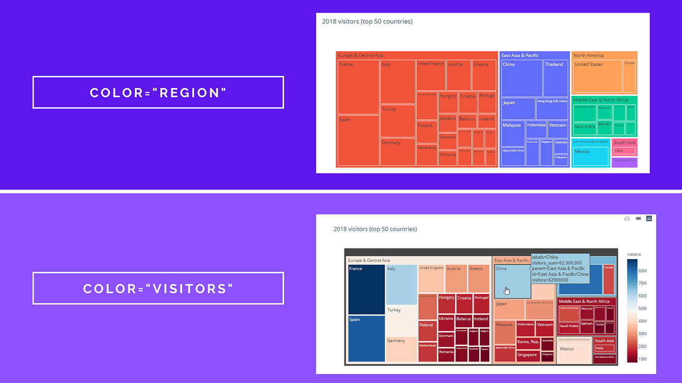
Treemap
If pie and sunburst charts are hard to read when you display a lot of data, the opposite is true for the treemap. You can play with the color and assign either a discrete scale based on a categorical column or a continuous scale.
Choropleth — Maps with plotly
We are looking at the data about the world and using maps is an obvious choice on how to display them. Plotly has some support for displaying geospacial data with build-in country shapes, regional scopes, and options to adapt the colors and other parameters.
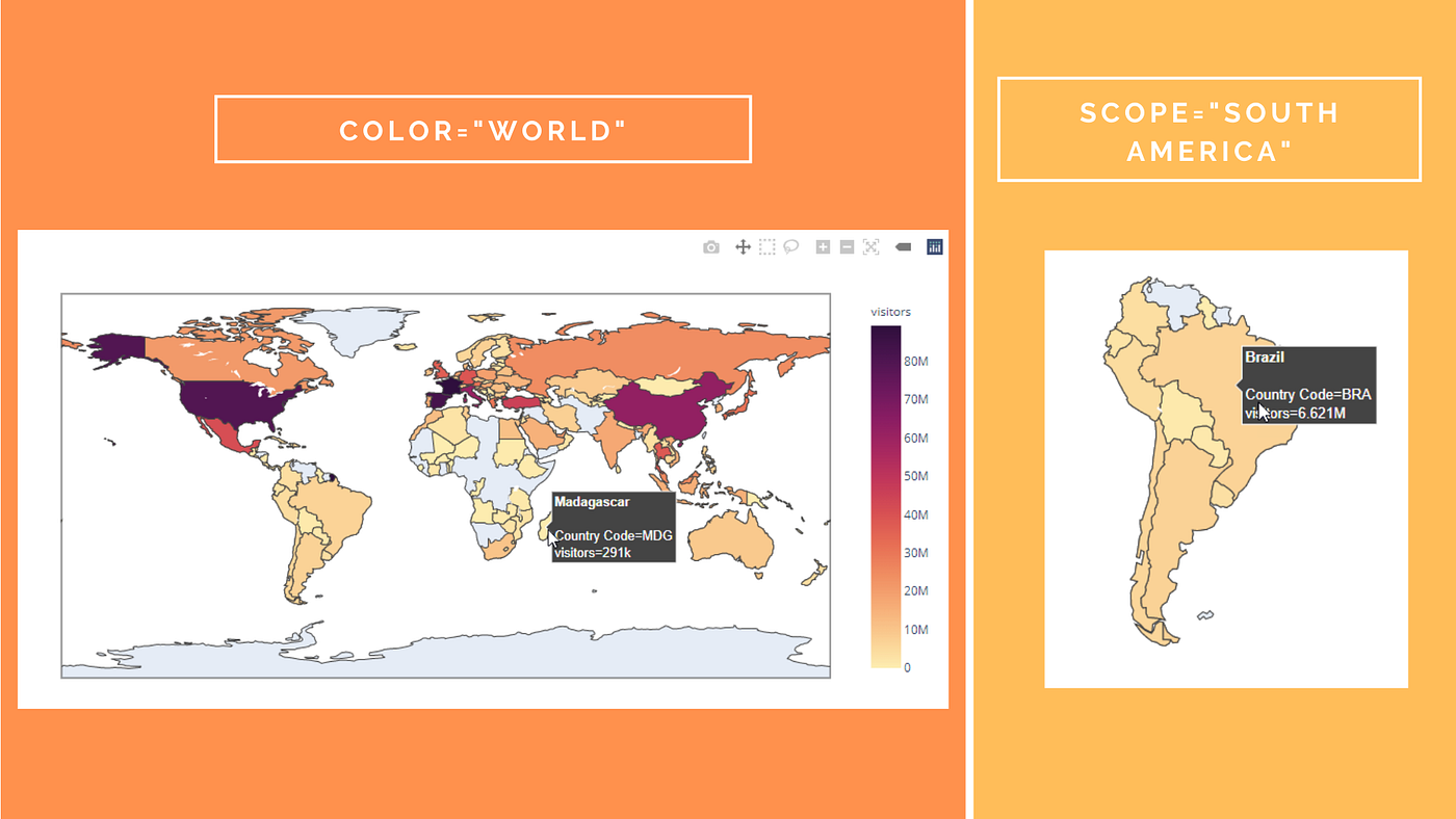
Based on the documentation, the countries are identified by ISO-3 Code, country name or US-State names. If you want to dig deeper you have to get your own
geojsoncoordinates of the geographical obejcts.
Scatter chart
Scatter plots are one of the most common types of plots. They can easily show relations between the two-dimensional data and using colors and sizes you can pack your visualization with even more information. We will however start where we have left. In the geography using scatter_geo graph.
            fig = px.scatter_geo(
              melted_df.fillna(0),
              locations ="Country Code",
              color="visitors",
              size="visitors",
              # what is the size of the biggest scatter point
              size_max = 30,
              projection="natural earth",
              # range, important to keep the same range on all charts
              range_color=(0, 100000000),
              # columns which is in bold in the pop up
              hover_name = "Country Name",
              # format of the popup not to display these columns' data
              hover_data = {"Country Name":False, "Country Code": False},
              title="International Tourism",
              animation_frame="years"
              )
fig.update_geos(showcountries = True)
fig.show() 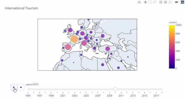
Important scatter_geo parameters are max_size allowing to set the biggest radius of the bubbles and opacity to determine how much of the plot is visible.
Scatter Plots
Regular scatter charts are commonly used to display the relation between the two variables. In our case, the number of visitors and their expenditures in the country. I will look only at the year 2018. size parameter influences the size of the bubbles while color parameter lets you set the color based on a categorical or continuous variable.

Scatter plots allow to easily add marginal plots to highlight the distribution of one variable or of several variables specified by the color argument. You can choose from 4 types of marginal plot — box, violin, histogram or rug. You set them up simply by applying marginal_x or marginal_y parameter e.g. marginal_x="rug". You can also draw a trend line for each color on the chart.
            px.scatter(df,
              x="visitors",
              y="receipts",
              color="type",
              hover_name="Country Name",
              size="receipts",
              marginal_x="histogram",
                marginal_y="box",
              trendline="lowess",
title="Scatter plot with histogram and box marginal plot and two trendlines") 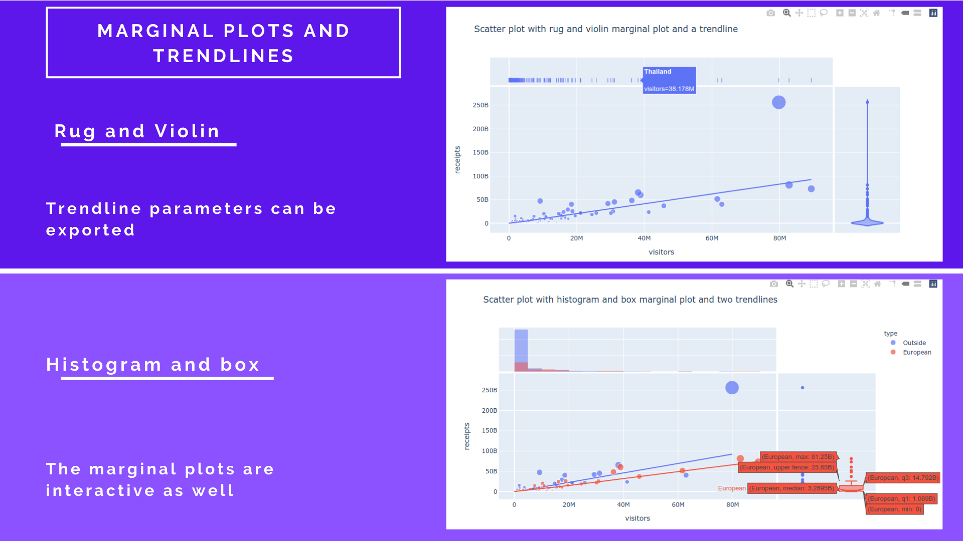
To draw trendlines you need to install statsmodel library
conda install -c anaconda statsmodels
# or
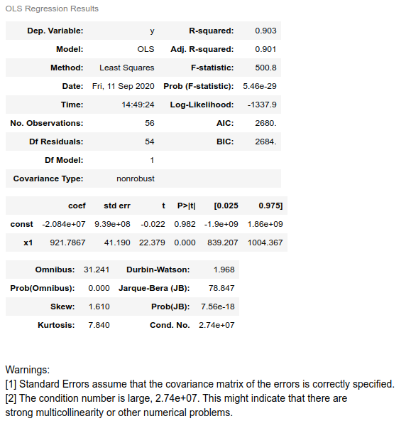
pip install statsmodels Thanks to statsmodels library you can also display the parameters of the regression model which was used to calculate the trendline.
            # get the parameters via `get_trendline_results`
res = px.get_trendline_results(fig)            # get the statsmodels data
[In]:
trendline = res["px_fit_results"].iloc[0]
print(type(european_trendline))            [Out]: <class 'statsmodels.regression.linear_model.RegressionResultsWrapper'>            # print the summary
trendline.summary()
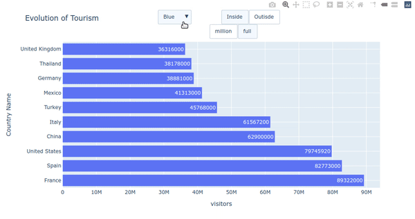
Interactive Buttons
Plotly's success can be attributed to interactive features. Each chart contains a menu in the top right corner which allows basic operations like zoom-in and out, what tooltip appears when you hover graphs' elements or you can save the plot as an image by a single click.
You can also add interactive buttons (or dropdowns) which let the users change the look of the graph. You can add four types of actions using parameter method:
-
restyle— to influence the look and feel of the data or the type of the chart -
relayout— to change the properties of the layout -
update— combines the two methods above -
animate— allow to control the animation features
You can put several groups of buttons on the chart. They can be arranged either next to each other (or on the top of each other) or as a dropdown.
Interactions
The documentation shows some basic interactions, but if you plan to do something else, it is quite tricky to achieve that. The best trick is to create final the look you want to reach, dump the dictionary using fig.to_dict() and copy the relevant sections of the dict into arg[{...}] of the button for example:
            # create the chart and export to dict
px.bar(df, x="visitors", range_x=[0,10]).to_dict()            # read the dict to find the relevant arguments for the update
# arg. xaxis.range of the relayout changes the x_range                          fig.update_layout(
              updatemenus=[
              dict(
              buttons=list([
              dict(
              args=[{"xaxis.range":[-2,10],
              "yaxis.range":[0,5.6]}],
              label="x:right 1, y:bottom 0",
              method="relayout",
              )]),
              type="buttons",
              showactive=True,
              x=1,
              xanchor="right",
              y=0,
              yanchor="bottom"
              )])            # see the full example on github for more ideas
See the github notebook for more ideas about what to do with the buttons or explore the examples in Plotly's documentation.
I have succeeded to change the labels, colors, ranges, but I have failed to change the input values (e.g. change the source data).
Buttons' position
You can place the buttons all around the plot area using the coordinate system, where x: 0, y: 0 is the bottom left corner of the chart (some plots like pie chart don't fill in whole area). You can also set the xanchor and yanchor to be left-center-right or top-middle-bottom.
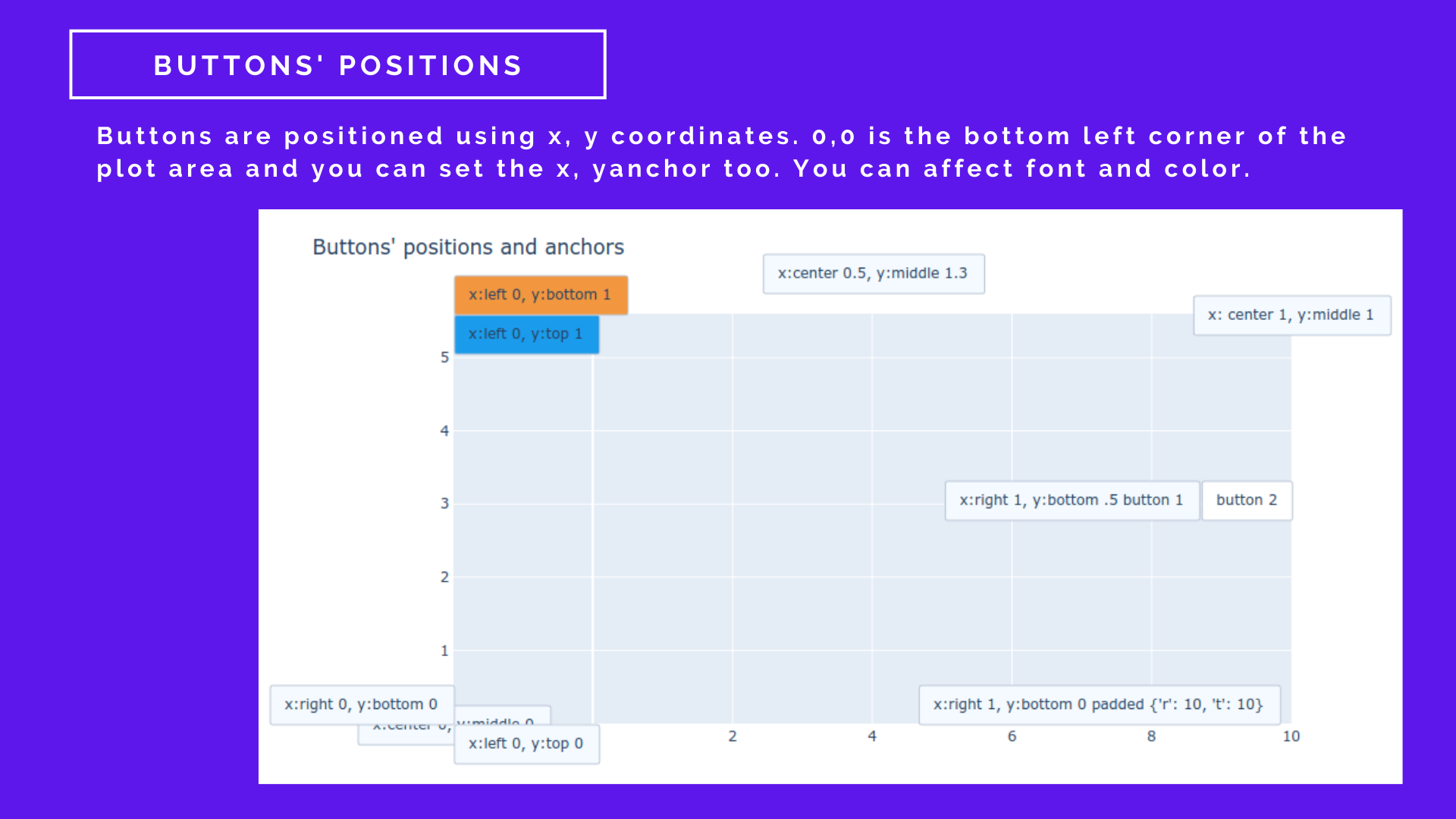
Clicking the buttons sometimes change their position
You can micro-adjust the position using pad={"r": 10, "t": 10}. The values are in pixels and you can pad r-right, l-left, t-top, b-bottom. You can also change the font and color of the buttons.
Export Plotly
You can export the generated chart either as an interactive HTML page which lets you do all the Plotly magic, like zooming, switching data on/off or see the tooltips.
fig.write_html(f"{file_name}.html") You can specify several parameters specifying whether 3MB plotly.js is included, if the animation starts upon opening or how the html document is structured— documentation.
You can also export the image as a static picture using .write_image(). It let you export into several formats like .png, .jpg, .webp, .svg, .pdf or .eps. You can change the dimensions and scales. Plotly is using kaleido as a default engine, but you can also choose a legacy orca engine.
            # install caleido
pip install -U kaleido
#or conda install -c plotly python-kaleido            # export the static image
fig.write_image(f"{file_name}.png")
Plotly as pandas default backend
You can set up Plotly as pandas default plotting backend.
pd.options.plotting.backend = "plotly" Then you apply the plotly parameters to the data frame itself.
            fig = df.plot(kind="bar", x="x", y="y", text="y")
fig.show()
It's however so easy it input the dataframe as the first parameter, that you might prefer pandas default set up having matplotlib as backend.
            # return to defaul matplotlib backend
pd.options.plotting.backend = "matplotlib"
A few pitfalls
Once you get yourself familiar with Plotly.Express you rarely come across an issue, you cannot solve. As we have said, Express struggle with the subplots. There are also some other situations that can increase your heartbeat. But even those have a simple solution.
If you want to display the value count of integer categories, e.g. how many times player number 1,2,3 won a medal, it's simple using standard padnas plotting with Matplotlib.
            """if you want to display which values are the most frequent and these values are integers"""            df = pd.DataFrame({"x": [3]*10+[6]*5+[2]*1})
df["x"].value_counts().plot(kind="bar")
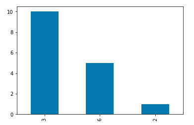
But if you try the same with Plotly, it automatically assumes that you want to display a continuous range of integers on the x-axis.
            """it's rather impossible with plotly which always set up the range containing all the numerical values"""            fig = px.bar(df["x"].value_counts())
fig.show()

To get the expected chart, you must turn the values into categories, though not in pandas.
df["y"] = df["y"].astype("category") # or .astype("string") You must change the axes in the Plotly's layout parameters:
            fig.update_xaxes(type="category")
fig.show() 
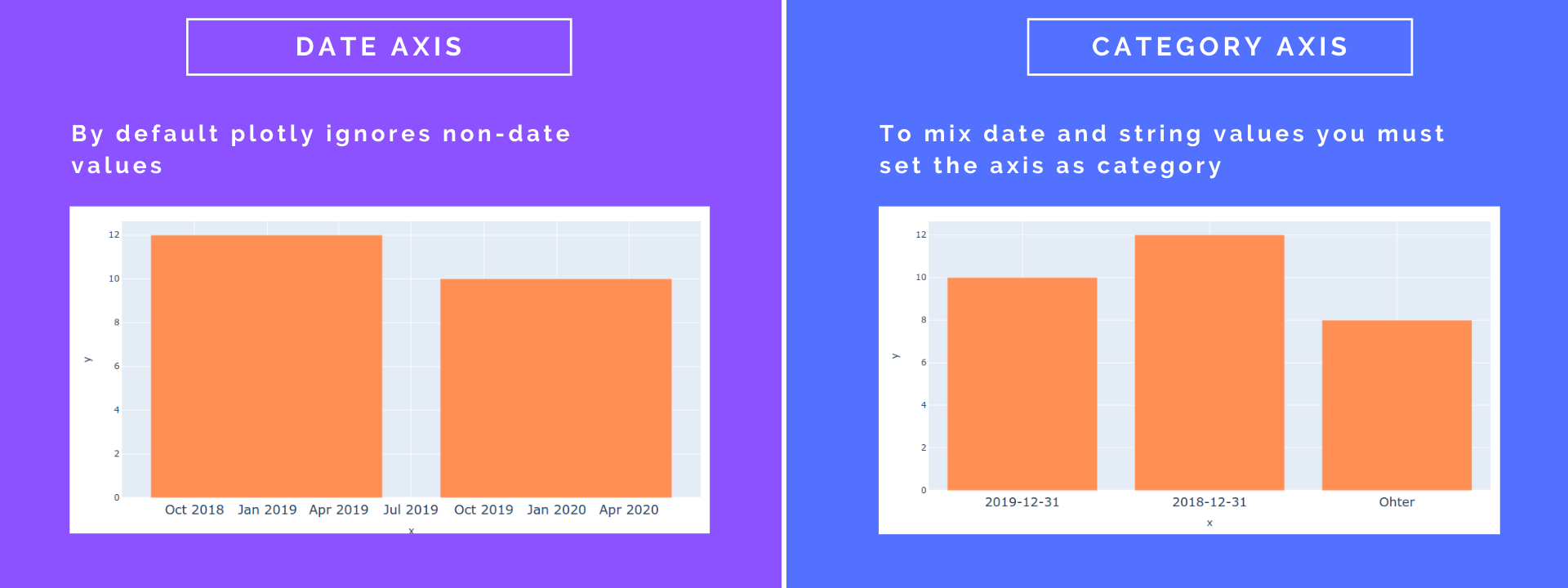
Plotly also automatically handles the date values, which is particularly annoying in the case of end-of-the-season (year/quarter).
            """Also the daterange labels on the x-axis can annoy you when you try to display end of the year/quarter dates.
Plotly will always turn them into the Jan next year or the beginning of the following quarter"""            df = pd.DataFrame({"x":["2019-12-31","2019-03-31","2018-12-31","2017-12-31"],
              "y":[10,12, 15, 8]})
fig = px.bar(df, x="x", y="y")
fig.show()
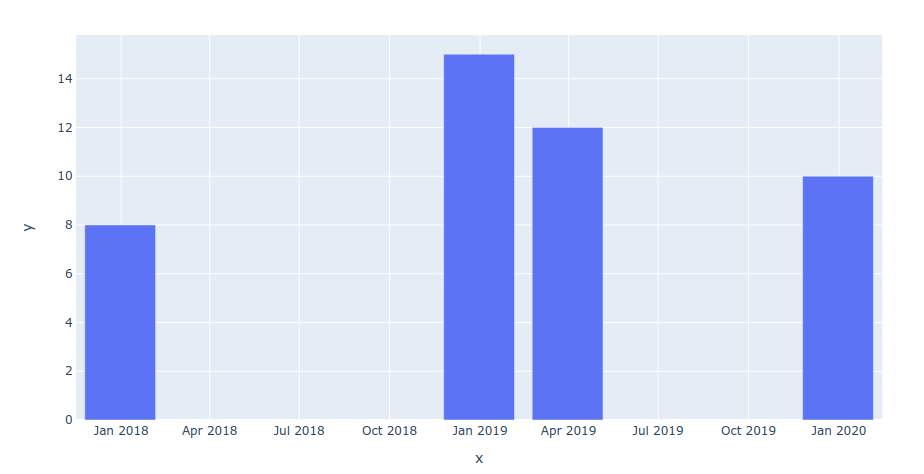
Plotly automatically scales the axis labels to show the distribution in time, but if you wanted to display the end-of-year (quarter) dates, you will be very disappointed seeing the beginning of the next year instead. In case you want to display e.g. companies' financial data at the end of each year and you see '2020' instead of 'End of 2019' and you can get a completely wrong impression about the company's health. The fix is the same fig.update_xaxes(type="category")
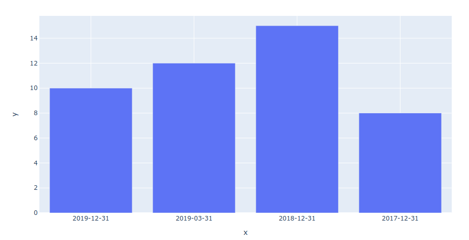
Plotly is clever, and once you populate the axis with a date it considers it a date axis. Sometimes you may want to really display date and string values on the same axis. Solution, yes .update_xaxes(type="category") again.
Documentation summarized
- Scatter Chart — API, Examples
- Line Chart — API, Examples
- Bar Chart — API, Examples
- Pie Chart — API, Example
- Sunburst Chart —API, Example
- Treemap Chart — API, Example
- Choropleth — API, Examples
- Scatter_geo chart— API, Examples
- Scatter Chart — API, Examples
- Histogram — API, Examples
- Trendlines
- Axes — API
- Text and Annotations — Examples
- Marginal Plots — Examples
- Export — write_html or write_image
- Buttons (Update Menus) — API, Examples
Conclusion
Plotly express is a great way how to quickly display your data using a single chart type. It has significant features like interactivity and animations but lacks the support of subplots. Express is clever, and it split your data frame with a logical subset of data most of the time. But if it makes a wrong guess, it's almost impossible to persuade Plotly to display the data the way you want.
Sometimes it requires a bit of trial and error. It usually helps to export the chart into a dict and try to find the correct name of the parameter you want to update. If you cannot create the desired visualization using Plotly.Express you can always alternate to the lower level API which is much more benevolent, but also requires more coding.
If you, on the other hand, need more complex interactive reports, you will opt for Dash a dashboard tool of Plotly, which requires a bit more coding but you can achieve a really professional-looking dashboard with Dash.
Resources:
Plotly 4.0.0 Release notes
            If you liked this article, check other guidelines:            * Highlighted line chart with plotly
* Visualize error log with Plotly
* All about Plotly Express Histograms
* How to split data into test and train set            All the pictures were created by the author.                        Many graphics on this page were created using canva.com (affiliate link, when you click on it and purchase a product, you won't pay more, but I can receive a small reward; you can always write canva.com to your browser to avoid this). Canva offer some free templates and graphics too.
The charts and the exercises are available in the Github repo. Feel free to try, update and change — Plotly Express — Comprehensive Guide.ipynb
How Yo Make Each Level.of Graph.different Color
Source: https://towardsdatascience.com/visualization-with-plotly-express-comprehensive-guide-eb5ee4b50b57
0 Response to "How Yo Make Each Level.of Graph.different Color"
Post a Comment